
Artificial neural networks for small dataset analysis
Introduction
Nowadays we have many examples of complex systems at macroscopic scale: the climate system, a number of ecosystems on the Earth, the global economic system, internet, etc. In any case, none of them gets close to the complexity of the human body, both considered as itself or, even more, together with its relationships with the surrounding environment.
As well known, the difficulties in describing and predicting the behaviour of these systems are deeply linked with the multiple connections of their constitutive elements and the many feedbacks arising from frequent cause-effect closed chains. All these characteristic features lead to a general nonlinear behaviour of these systems, more or less close to a linear one, depending on their “status” and the values of certain critical thresholds.
In this situation, a dynamical description of these systems is generally very difficult and sometimes impossible. Thus, data-driven methods have been worked out for possibly disentangling their skeins and achieving correct information about cause-effect relationships, especially about the final effects of external/environmental forcings on the behaviour of the systems themselves. Obviously, statistical methods are usually involved in these attempts to extract knowledge, from the simplest techniques, such as correlation and regression analyses, up to the most sophisticated ones.
In this framework, as we will see, modelling a complex system (or the relationships between this system and its external environment) by artificial neural networks (ANNs) gives the possibility to fully take nonlinearities into account, even without considering the number of closed loops present in the system itself and their complex interactions and balance.
At present, ANNs are developed and used in many fields of the contemporary scientific research, with several different purposes. Here, I limit to describe and apply a basic kind of ANNs—the feedforward networks with backpropagation training—which is able to perform realistic nonlinear multiple regressions in a reliable manner, if applied correctly. Here, “realistic” means that the regression “law” found is a reasonable one and is not affected by problems which frequently arise in nonlinear systems, such as overfitting. On the other hand, “reliable” means that the results can be considered robust and are not affected by variabilities inside the network structure. Obviously, all these considerations will appear clearer when ANNs will be formally introduced and then applied to concrete case studies.
Data-driven models—and especially artificial intelligence methods—have been recently considered as the fundamental tool for achieving knowledge in a big-data environment (1). Without entering into the debate on this topic, I would like to stress that, if we exclude large epidemiological studies, frequently in health sciences we have to do with short series of data, rather than with long ones. Thus, a technique which allows us to handle a small-data nonlinear environment is perhaps more useful. In what follows, I will introduce and apply a specific ANN tool for extracting knowledge from a limited observational or experimental landscape.
In doing so, I first describe structure and functioning of feedforward ANNs with backpropagation training (Section 2), then going towards the introduction of a specific ANN tool for analyzing small datasets (Section 3). In this framework, in Section 4 a specific application of ANNs is presented and discussed, also introducing some interesting preliminary analysis which could drive the networks to more performant results, for instance through data preprocessing from previous knowledge of the system under study. Finally, brief conclusions are drawn.
Feedforward neural networks with backpropagation training
As easily understandable, the development of ANN models has been clearly inspired by neurosciences: see (2,3) for an historical introduction to this field and for the fundamentals of the networks presented in this Section. At present, of course, there are many studies about a detailed simulation of neurons and their connections in the animal and human brains via ANNs. However, the ANN models presented here do not aim to be biologically realistic in detail, but they are chosen uniquely for their ability to find nonlinear realistic relationships between some causes and some indices which summarize the behaviour of a certain complex system.
In doing so, I deal explicitly with feedforward neural networks, which are the most applied to environmental and health studies, even if many distinct kinds of network models have been obviously worked out: see (4,5) for other examples and their applications.
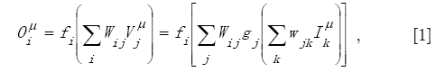
More specifically I will describe the structure and functioning of a “multilayer perceptron” with one hidden layer and one output (see Figure 1, where this kind of network is depicted together with the notations used in this paper). This is a quite standard tool for studying cause-effect relationships in a complex system, with the purpose of reconstructing the behaviour of a certain variable starting from knowledge of other (causal) variables which we estimate to be important for driving its evolution. The limitation to just one layer of hidden neurons is justified by the fact that one hidden layer is enough to approximate any continuous function (6,7).

The fundamental elements of the network are the connections, with their associated weights (wjk and Wij), and the neurons of the hidden and the output layers, which represent the single computational units (they calculate the result obtained by the application of an activation function to the weighted sum converging at the neuron: see eq. [1] in what follows). In this architecture of the network each neuron is connected to all the neurons of the previous and the following layer; there are no connections between the neurons on the same layer.
If we consider the inputs as some causes which drive the output (our effect), it is clear that our aim is to find a transfer function that correctly leads from inputs to the correct output behaviour (the so-called “target”). As a matter of fact, once fixed the weights, the nonlinear functions gj calculated by the hidden neurons and the linear function fi calculated at the output neuron, this network is able to do so. In fact, in the general case of multiple outputs, the i-th output is given by:
where:
 = inputs (usually normalized between 0 and 1, or -1 and 1);
- wjk = connection weights between input and hidden layers;
- Wij = connection weights between hidden and output layers;
 = output of the hidden neuron Nj = input element at the output neuron Ni;
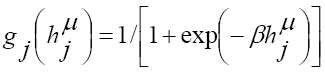 (for inputs normalized between 0 and 1) or
 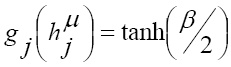 (for inputs normalized between -1 and 1), with the steepest parameter β which is often set to 1;
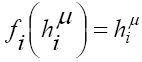 ;
; and
and  are weighted sums implicitly defined in eq. [1].
 = inputs (usually normalized between 0 and 1, or -1 and 1);
 = output of the hidden neuron Nj = input element at the output neuron Ni;
 (for inputs normalized between 0 and 1) or
  (for inputs normalized between -1 and 1), with the steepest parameter β which is often set to 1;
 ;
; and
and  are weighted sums implicitly defined in eq. [1].
As cited above, eq. [1] is written for the general case of multiple outputs. In our case of a single output i =1.
As evident from eq. [1], the output depends critically on the values of the weights wjk and Wij, exactly as in a multiple linear regression the value of the dependent variable y depends on the values of the coefficients associated to the linear terms of the independent variables x, z, t, etc. Thus, in order to find a successful “regression law”, as in a multiple linear regression we minimize the distance between the specific values of y and the real data, also in a nonlinear regression performed by an ANN we must minimize the distance between our reconstructions (outputs) of the observational or experimental data and the data themselves. Thus one tries to minimize the following squared cost function
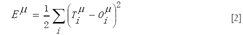
for every input-target pair (pattern) µ, where  (the targets) represent our observational data of a certain variable which summarizes the real behaviour of the system under study, and
  are the results of our ANN model.
While this minimization activity is quite trivial for linear regressions, in our multiple nonlinear cases it is a critical one. Several methods have been developed for approaching this problem. Here, I briefly describe an iterative procedure, the so-called error backpropagation training.
First of all, one randomly chooses a set of initial weights. Then he applies eq. [1] in a forward step, so finding an output. At this point, an estimation of Eµ can be performed. Usually the values of target and output can be very distant and our reconstruction unsatisfying. Thus one searches for the minimum of eq. [2] by means of a backward step in which he changes the values of the weights via the following rules:
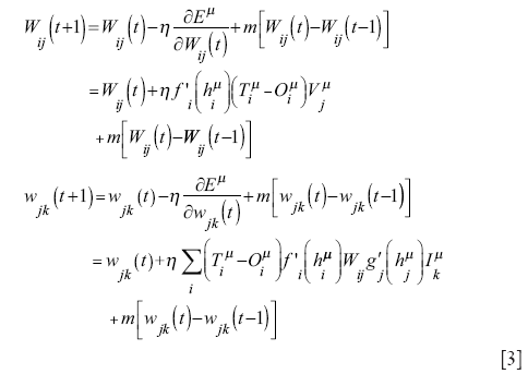
Here η is the so-called learning rate, which determines the amount of the term, coming from the minimization of the cost function via a gradient-descent rule, which our model takes into account. This term allows the model to climb down the valleys of the landscape of the cost function (shown in Figure 2) towards a minimum. m is the so-called momentum coefficient: it represents the “inertia” of this method and is very useful in order to avoid entrapment of the solution in a local minimum, because it permits to jump over them, leaving the possibility to achieve the absolute minimum (Analogous equations can be applied to the update of the so-called thresholds of the neurons. The threshold, or bias, is an internal value of each neuron, which is subtracted from the total input before computating the functions g and f. The use of these thresholds permits to limit the value of the total input. Here, I have omitted any thresholds from this formal description, because they can always be treated as further connections linked to an input neuron that is permanently clamped at 1. Therefore, the update of the threshold weights can be performed through equations similar to eq. [3].).

At this point, a new forward step with the new values of weights can be performed, finding a new estimation of Eµ. Successive backward-forward cycles can be performed till the desired accuracy in estimation will be achieved, for instance under a certain threshold S:
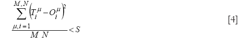
where M is the number of input-target pairs (patterns) and N is the number of output units.
However, an ANN is so powerful that it is able to obtain a nonlinear function that reconstructs in detail the values of targets starting from data about inputs if every input-target pair is known to it, and a large number of neurons in the hidden layer are allowed. But in this case, ANNs overfit data and no realistic regression law can be obtained (Here, the number of hidden neurons is the analogue of the degree of the polynomial in a polynomial regression for fitting experimental data. If you have 100 experimental data on a Cartesian plan, you can always fit them perfectly by a polynomial of degree 99, but nobody can say that it represents a natural law. In fact, if you try to fit other data from another sample of the same population, you obviously see that the score of this high-degree polynomial is lower than that of a low-order one: we have overfitted our sample). Thus, we have to consider only a small number of hidden neurons and, at the same time, we must exclude some input-target pairs from the training set on which the regression law is built. Only if the map derived from the training set is able to describe the relation between inputs and target even on independent sets can we say that a realistic regression law has been obtained.
An ANN tool for analyzing small datasets
In the backpropagation framework previously described, the number of hidden neurons is taken low [a few theoretical rules and many empirical methods are used for this—see, for instance, (8)] and a training-validation-test procedure is usually adopted for the optimization of an ANN model.
In short, the entire sample of data is divided into three subsets (Figure 3). First of all, the backpropagation algorithm is applied on a training set, then, at each step of iteration, the performance of the obtained input-output map is validated on distinct data (the so-called validation set), by considering a forward step from the inputs of the latter set to their outputs, through a network with the weights fixed at this step by the backpropagation method on the training set. The iteration process is stopped when the performance on the validation set begins to decrease, even if the performance on the training set continues to increase under certain desired thresholds (see Figure 4). This procedure, called early stopping, is performed to avoid the overfitting due to a too much close reconstruction of the data in the training set. Finally, a test set of data, completely unknown to the network, is considered. Just on this test set one can measure the real performance of the ANN model in reconstructing (in many cases, forecasting) new data and events.


In this way we are generally able to obtain realistic nonlinear transfer functions between variables that may be linked by cause-effect relationships in a complex system. In order to do so, however, we need a big sample of data available. If this is not the case, as often happens in health studies, the exclusion from the training activity of the data contained in both validation and test sets can lead to exclude peculiar behaviours of the system which may be not represented in the training set: obviously, this undermines the general validity of the regression law found.
In order to avoid this problem, an ANN tool including a particular training-validation-test procedure for small datasets has been developed some years ago and recently refined in order to obtain not only realistic regression laws, but also reliable ones. One can refer to (9,10) for the fundamentals of this tool, to (11-13) for some recent applications to problems characterized by limited data, and to (14) for the updated version of the specific procedure cited above.
The fundamental idea for dealing with small datasets is to maximize the extension of the training set by a specific facility of the tool, the so-called all-frame or leave-one-out cross validation procedure. Here I refer directly to the generalized version of this procedure first introduced in (14): see Figure 5 for a sketch of it.

In short, each target is estimated—we obtain an output—after the exclusion of the corresponding input-target pair (pattern) from the training and validation sets used to determine the connection weights. Referring to Figure 5, the white squares represent the elements (input-target pairs) of our training set, the black squares represent the elements of the validation set and the grey square (one single element) represents the test set. The relative composition of training, validation and test sets changes at each step of an iterative procedure of training, validation and test cycles. A ‘hole’ in the complete set represents our test set and moves across this total set of pairs, thus permitting the estimation of all output values at the end of the procedure. Furthermore, the validation set is randomly chosen at every step of our procedure and the training stops when an increase in the mean square error (MSE) in the validation set appears. This new procedure allows us to definitely avoid any overfitting on data we want to reconstruct by ANNs.
Obviously, the results of this generalized leave-one-out procedure critically depend on the random choices regarding both the initial weights and the elements of the validation set. For taking this fact into account and obtaining more robust results, we can perform ensemble runs of the ANNs, by repeating a certain number of times (usually 20-30) every estimation shown in Figure 5 with new random choices for both the weights and the elements of the validation set. In particular the change in the values of the initial weights allows the model to widely explore the landscape of every cost function, starting from different initial points in the multidimensional analogue of Figure 2.
When one averages on these multiple (ensemble) runs of the model, he is able to obtain results which are more robust and reliable, because they do not depend on the variabilities connected with the network initialization and with the random choice of the validation set.
An example of application
Since the last decade of the twentieth century, several applications of ANNs have been performed in medical sciences: see, for instance, (15-17) and references therein. There was a wide range of applications, from epidemiological studies to technical analyses of EEGs, from the standard topics of medical sciences to genetics. In any case, the adoption of ANNs led to some kind of improvement in our knowledge of the topic considered, due to the accurate handling of data about a certain nonlinear subsystem of our body, possibly in interaction with its internal and external “environment”.
Here, I would like to show how to apply the tool previously described in order to study the possible causes of illness events, also giving a concrete example in the area of thoracic disease, where the tool itself has been already used (18).
In general, when dealing with a complex system, its behaviour can be driven by many causes. The onset of a disease, for instance, may be due to a particular combination of causal factors. This is particularly evident for some thoracic diseases, due to the direct interaction of the respiratory apparatus with external factors, such as different values of meteorological parameters and pollutants.
In this framework, ANNs can help us to identify the possible causes and their peculiar combination linked to the onset of a certain disease, especially in cases in which we do not possess a clear knowledge of the dynamical relationships among these factors. This is properly the case for the onset of the Primary Spontaneous Pneumothorax (PNP) studied in (18) by the ANN tool previously described. Here I do not enter into details of that study, but take it as a concrete case to explain which steps can be done when applying an ANN model. For further details on this specific application, see (18).
The first step is to try to understand which causal factors may be prominent. A quite standard method adopted for this is the linear correlation analysis through calculation of the so-called Pearson’s correlation coefficient R. But here the system shows nonlinearities, so this method is not able to assess possible nonlinear relationships among variables.
Thus, a preliminary statistical analysis can be performed in order to explore if linear and nonlinear correlations among the variables of interest have the same magnitude: in this way we assess if a fully nonlinear method can lead to differences (hopefully, improvements) in the description of the system. If we use a neural network jargon, we can call “inputs” the variables used in order to model the investigated behaviour of our system, for instance the onset of a disease (which is our “target”). Now we can compare the relative importance of inputs by means of linear and nonlinear bivariate analyses against the target. Here we use the standard linear correlation coefficient R and its nonlinear generalisation Rnl, the so-called correlation ratio, whose square can be written as (10,19):
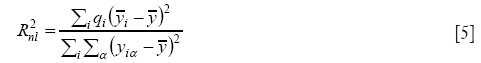
We can consider the target (the PNP daily cases, in our study on PNP) as the dependent variable and one input at a time (daily meteorological parameters and pollutant concentrations) as the independent variable. Then we group the values of the input into classes. Here Rnl is defined in terms of the average of the target for every specific ith class of the chosen input: in fact, qi is the sample size for the ith class of the input, 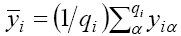 is the average of target for the ith class of the input,
 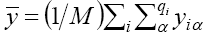 is the average of target on all the classes of the input and
 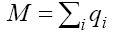 is the total size of the set here considered. Of course, the value of Rnl depends on the number of classes considered: the more reliable value can be obtained for the maximum number of classes that allows us to obtain a smooth histogram.
In doing so, in general one founds differences between linear and nonlinear correlation values for the same input-target sets; in particular, he is able to discover that inputs having low linear correlation with the target sometimes assume high nonlinear correlation values.
Even if the correlation ratio does not measure all types of nonlinearity, calculations of Rnl on our PNP problem allowed us to understand that some nonlinearities are hidden in the relationships among the variables considered there. Furthermore, as a consequence of these bivariate analyses, the inputs to be considered for an optimal ANN nonlinear regression could be generally different from the variables chosen for an optimal linear regression.
After this preliminary analysis one is able to determine the most important single input variables for a successful reconstruction of the target behaviour. However, a further attention must be required in view of the development of a model which is able to do so by considering several inputs. In fact, even input variables which are highly correlated with the target can lead to poor results once inserted in an ANN model, if they show high absolute values of R or Rnl between them. In this case, in fact, these variables carry almost the same information and the ANN model shall not benefit from their joint consideration.
After this input selection, one can build several models characterized by different inputs, so performing nonlinear multiple regressions via ANNs and finding the best configuration of causal variables that permits to explain the maximum variance in the target behaviour. Due to the nonlinear nature of the system under study, only a model such as that described here is able to account for the combined nonlinear influence of a set of causal variables on a particular effect (our target).
In datasets characterized by short records one can then apply the generalized leave-one-out procedure previously introduced. In this manner, he is able to identify the most important causal variables and to reconstruct at best the onset of a disease. This ANN model with fixed weights can be obviously applied to forecast future cases, once the values of the causal input variables can be predicted (for instance, day by day).
In this specific application, the ANN model has been applied without any use of our previous knowledge of the relationships between inputs and target. Sometimes, however, our expertise can be used for making easier the task of an ANN model. For instance, if the target and some inputs undergo a day-night cycle, the cycle itself may be “subtracted” from the series before putting their residual data into the network. Refer to (20) for a case of this kind. It has been shown that this use of our previous knowledge can lead to better results with respect to the previous direct application. In particular, the ANN model is often able to find a “dynamics” in the residual target behaviour even if it can appear as a random one.
Finally, it is worthwhile to say something about what we may intend for small dataset. In general, there is no threshold for the amount of data we can consider as small. This concept is not autonomous, but it is related to the size of the ANN we would like to use for modelling the system under study.
Due to the necessity to avoid overfitting, some empirical rules [see (8) for more details] must be applied to our analysis. In particular, we should require that the number of patterns is at least one order of magnitude more numerous than the number of connections of the network (including threshold ones). Given the number of inputs, this rule allows us to calculate how many neurons may be considered in the hidden layer without falling into overfitting conditions.
As a last remark, I cite that the performance of an ANN model can be estimated by several methods, as indicated, for instance, in (21), from the continuous ones, till those characterized by thresholds. Typical is the use of contingency tables and the related performance measures: probability of detection, false alarm rate, Heidke’s skill score, relative operating characteristic (ROC) curve, etc.
Conclusions
In this paper, I tried to introduce the reader to a kind of neural network models which is particularly useful in analyzing nonlinear behaviours in small datasets, with the aim of finding causal relationships. The specific tool described here has been extensively tested on environmental problems and recently used in the analyses of a thoracic disease, too. This tool is also implemented in MATLAB® and this version is available on request for collaborations or independent use after citation.
I hope that this brief review could push some researchers in the field of health sciences to adopt neural networks as a powerful instrument for disentangling the complexity of their subject matter.
Acknowledgements
Disclosure: The author declares no conflict of interest.
References
- Anderson C. The end of theory: the data deluge makes the scientific method obsolete. Wired 2008;16. Available online: http://archive.wired.com/science/discoveries/magazine/16-07/pb_theory
- Hertz J, Krogh A, Palmer RG. Introduction to the theory of neural computation. New York: Addison-Wesley Longman Publishing Co., 1991:327.
- Bishop CM. Neural networks for pattern recognition. New York: Oxford University Press, 1995:482
- Haupt SE, Pasini A, Marzban C. Artificial intelligence methods in the environmental sciences. New York: Springer, 2009:424.
- Hsieh WW. Machine learning methods in the environmental sciences. Cambridge: Cambridge University Press, 2009:364.
- Cybenko G. Approximation by superposition of a sigmoidal function. Mathematics of Control, Signals, and Systems 1989;2:303-14.
- Hornik K, Stinchcombe M, White H. Multilayer feedforward networks are universal approximators. Neural Networks 1989;2:359-66.
- Swingler K. Applying neural networks: a practical guide. London: Academic Press, 1996:303.
- Pasini A, Potestà S. Short-range visibility forecast by means of neural-network modelling: a case-study. Il Nuovo Cimento C 1995;18:505-16.
- Pasini A, Pelino V, Potestà S. A neural network model for visibility nowcasting from surface observations: Results and sensitivity to physical input variables. J Geophys Res 2001;106:14951-9.
- Pasini A, Lorè M, Ameli F. Neural network modelling for the analysis of forcings/temperatures relationships at different scales in the climate system. Ecological Modelling 2006;191:58-67.
- Pasini A, Langone R. Attribution of precipitation changes on a regional scale by neural network modeling: a case study. Water 2010;2:321-32.
- Pasini A, Langone R. Influence of circulation patterns on temperature behavior at the regional scale: A case study investigated via neural network modeling. J Climate 2012;25:2123-8.
- Pasini A, Modugno G. Climatic attribution at the regional scale: a case study on the role of circulation patterns and external forcings. Atmospheric Science Letters 2013;14:301-5.
- Papik K, Molnar B, Schaefer R, et al. Application of neural networks in medicine – a review. Med Sci Monit 1998;4:538-46.
- Patel JL, Goyal RK. Applications of artificial neural networks in medical science. Curr Clin Pharmacol 2007;2:217-26. [PubMed]
- Shi L, Wang XC. Artificial neural networks: Current applications in modern medicine. IEEE 2010:383-7.
- Bertolaccini L, Viti A, Boschetto L, et al. Analysis of spontaneous pneumothorax in the city of Cuneo: environmental correlations with meteorological and air pollutant variables. Surg Today 2015;45:625-9. [PubMed]
- Marzban C, Mitchell ED, Stumpf GJ. The notion of “best predictors”: an application to tornado prediction. Wea. Forecasting 1999;14:1007-16.
- Pasini A, Ameli F. Radon short range forecasting through time series preprocessing and neural network modeling. Geophysical Research Letters 2003;30:1386.
- Marzban C. Performance measures and uncertainty. In: Haupt SE, Pasini A, Marzban C. eds. Artificial intelligence methods in the environmental sciences. New York: Springer, 2009:49-75.

